How to Plan a Serial Dilution Without Making Errors

Serial dilution is one of the most common techniques in a wet lab — and one of the most common sources of silent, systematic error.

The math is simple. The planning is not.

What is a Serial Dilution?

A serial dilution is a step-wise reduction in concentration where each step uses the output of the prior one as the new stock solution. This controlled reduction in concentration is common in microbiology, enzyme assays, and analytical quantification protocols. As defined in the ScienceDirect serial dilution overview, serial dilution is a fundamental technique for producing a geometric concentration series from a single stock, enabling precise quantification across many orders of magnitude. The Wikipedia article on serial dilution further describes it as a process of diluting a solution in a stepwise fashion, typically by a constant factor (such as 10× or 2×) at each step, producing a logarithmic concentration series. For a thorough practical overview, see INTEGRA’s guide to serial dilutions and calculations.

How serial dilutions are performed — a brief procedural summary:

• Prepare labeled tubes containing a pre-measured volume of diluent (buffer, water, or media)
• Transfer a fixed volume from the stock into the first tube and mix thoroughly
• Transfer the same fixed volume from Tube 1 into Tube 2, mix, and change tips
• Repeat for each subsequent stage, always transferring from the previous tube
• Verify labels and volumes at each step before proceeding to the next stage

Serial dilutions are used across a wide range of laboratory workflows, including:

• Microbiology — counting bacterial colonies by diluting a culture to a workable density
• Immunology — preparing antibody titration series for ELISA or Western blot
• Pharmacology — generating dose-response curves across several orders of magnitude
• Molecular biology — creating DNA or RNA standard curves for qPCR
• Biochemistry — preparing enzyme substrate gradients for kinetic assays

The reason serial dilution is necessary is practical: pipettes have limits. A P10 can deliver as little as 1 µL. A P1000 maxes out at 1 mL. No pipette can deliver 0.005 µL — which is exactly what a direct 1,000,000× dilution from a 10 mM stock to 10 nM would require.

Serial dilution solves this by introducing one or more intermediate concentrations, each achievable with a pipette you actually have.

The Core Formula at Each Stage

Every stage of a serial dilution is just C₁V₁ = C₂V₂:

C₁ × V₁ = C₂ × V₂
V₁ = (C₂ × V₂) / C₁

Where:

• C₁ = concentration of the input solution (your current stock or intermediate)
• V₁ = volume to transfer (what you’re solving for)
• C₂ = target concentration for this stage
• V₂ = final volume of this stage

The solvent volume is simply:

V_solvent = V₂ − V₁

This applies identically at every stage. The challenge isn’t the algebra — it’s choosing C₂ and V₂ wisely.

Typical Serial Dilution Workflow

Before diving into the planning decisions, it helps to see the standard procedural skeleton. The ASM Microbe Library serial dilution protocol describes the following general workflow, which applies across most bench contexts:

1. Label all tubes before pipetting — include concentration, date, and reagent name. Mislabeled intermediates are a leading cause of protocol failure.
2. Prepare the diluent — add the correct volume of diluent (buffer, water, or media) to each tube before transferring sample. This ensures the final volume is correct and reduces pipetting steps at the bench.
3. Transfer from the most concentrated tube first — pipette the calculated transfer volume from the stock into Tube 1 (your first intermediate), mix thoroughly, then change tips.
4. Carry the dilution forward — transfer from Tube 1 into Tube 2, mix, change tips, and repeat for each subsequent stage.
5. Verify volumes and labels at each step before proceeding — a quick check takes seconds; recovering from a mislabeled intermediate does not.
6. Discard or store intermediates as appropriate — intermediates are often discarded after the final stage unless the protocol requires them for independent use.

This workflow is consistent across microbiology, immunology, and analytical chemistry applications. The planning decisions described in the rest of this article determine what goes into steps 2–4: which concentrations, which volumes, and which pipettes.

Why Intermediate Concentration Choice Matters

The intermediate concentration determines the dilution ratio at each stage. And the dilution ratio determines whether the transfer volumes are pipettable.

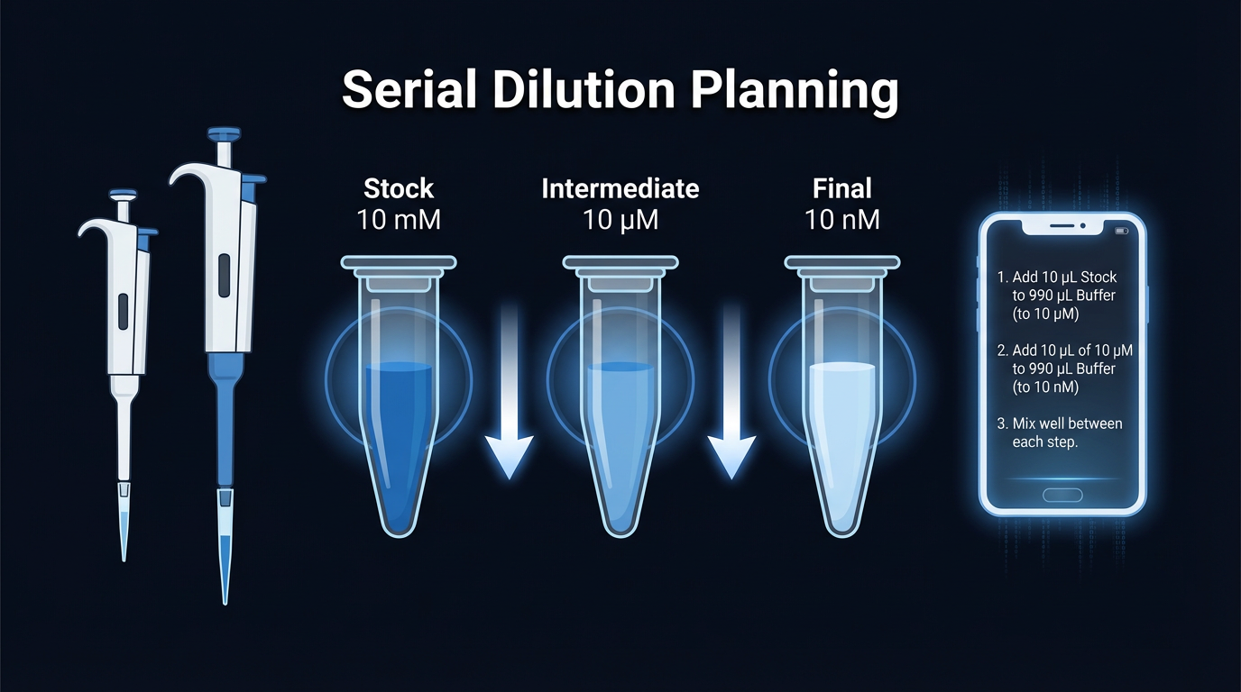
Consider a 10 mM → 10 nM dilution (1,000,000×). You need to split this into two stages. A few options:

Intermediate	Stage 1 ratio	Stage 2 ratio
10 µM	1,000×	1,000×
100 µM	100×	10,000×
1 µM	10,000×	100×

All three produce the correct final concentration. But they’re not equivalent in practice.

The 10 µM intermediate splits the work evenly: 1,000× at each stage. For a 1 mL final volume, Stage 1 requires a 10 µL transfer (P20 range), and Stage 2 also requires a 10 µL transfer. Both are comfortable.

The 100 µM intermediate makes Stage 1 easy (100×, large transfer) but Stage 2 brutal: 10,000× means a 0.1 µL transfer for a 1 mL final volume — below any standard pipette’s minimum.

The 1 µM intermediate has the same problem in reverse.

The principle: choose an intermediate that keeps transfer volumes in the comfortable range of your available pipettes at every stage.

Pipette Comfort Ranges

Not all pipettable volumes are equally accurate. Every pipette has:

• Hard range — absolute min/max the pipette can physically deliver
• Optimal range — where the manufacturer guarantees best accuracy
• Resolution — the smallest increment (P10/P20: 0.1 µL; P200: 1.0 µL; P1000: 10.0 µL)

A P10 at 10 µL is at its absolute maximum. The plunger is fully depressed and mechanical imprecision is magnified. A P20 at 10 µL is comfortably within its optimal range (5–18 µL). Same volume, meaningfully different accuracy.

When planning a serial dilution, you want every transfer to fall in the middle of a pipette’s optimal range — not at the edges. This is the same principle behind mid-range comfort scoring used in LabCalcPro’s pipette selection algorithm.

Pipetting Technique and Reproducibility

Good technique at the bench is as important as good planning on paper. Even a correctly designed protocol will produce inaccurate results if pipetting introduces systematic error at each stage. In a serial dilution, these errors compound: a systematic under-delivery in Stage 1 shifts the intermediate concentration, and Stage 2 amplifies that error into the final solution.

Common Error Sources

Common pipette calibration errors that affect serial dilution accuracy:

• Uncalibrated pipettes — pipettes drift over time and with heavy use. A pipette that reads 10 µL may be delivering 9.6 µL. Regular calibration (typically every 3–6 months, or per institutional protocol) is the only way to know.
• Wrong tip type — using non-manufacturer tips changes dead volume and aspiration characteristics. Always use tips rated for your pipette model.
• Tip not fully seated — an improperly seated tip creates an air gap that causes under-aspiration. Press firmly until you feel a positive stop.
• Pipetting at the wrong angle — angles greater than 20° from vertical cause liquid to contact the piston, introducing contamination and volume error.
• Not pre-wetting the tip — the first aspiration into a dry tip is systematically low; tip walls absorb a small amount of liquid on first contact.
• Temperature differences — thermal expansion affects volume accuracy. Allow cold reagents to equilibrate before pipetting.

Best Practices

Per INTEGRA’s serial dilution best practices guide and BPS Bioscience’s serial dilution protocol guidance:

• Pre-wet tips before every aspiration — aspirate and dispense 2–3 times before the actual transfer. Especially important for small volumes (< 20 µL) and aqueous solutions.
• Maintain consistent angle and immersion depth — hold ≤20° from vertical; immerse the tip only 2–3 mm into the liquid surface.
• Use forward pipetting for standard aqueous buffers — depress to the first stop to aspirate, then fully to the second stop to dispense.
• Mix each intermediate completely before drawing from it — pipette up and down 5–10 times or vortex for 3–5 seconds. An unmixed intermediate has a concentration gradient.
• Change tips between every stage — even 0.1 µL carryover can meaningfully shift a 1,000× dilution.
• Label intermediates immediately — include concentration and date before you pipette into the tube.
• Work at consistent temperature — allow cold reagents to equilibrate to room temperature before pipetting.

Quick Reference

Error source	Consequence	Fix
Dry tip	Under-aspiration	Pre-wet 2–3×
Wrong angle	Volume error + contamination	≤20° from vertical
Incomplete mixing	Concentration gradient in intermediate	Pipette 5–10× or vortex
Tip carryover	Concentration error propagates forward	Fresh tip every stage
Uncalibrated pipette	Systematic volume offset	Calibrate every 3–6 months

Rounding Propagates Through Stages

Here’s where many manual plans go wrong: they calculate ideal transfer volumes but don’t account for pipette resolution.

If Stage 1 calls for a 9.7 µL transfer on a P20 (resolution: 0.1 µL), the actual pipetted volume is 9.7 µL — fine. But if it calls for 9.73 µL, the pipette rounds to 9.7 µL. That 0.03 µL error changes the actual intermediate concentration slightly, and Stage 2 is now working from a slightly-off stock.

In a two-stage dilution, rounding errors at Stage 1 compound into Stage 2. The final concentration may be off by more than either rounding error alone.

A rigorous protocol accounts for this: it rounds transfer volumes to pipette resolution before computing solvent volumes, so the stated volumes are exactly what you’ll pipette. This is one of the core reasons LabCalcPro’s Show Math separates pre-rounding and post-rounding values — so you can see exactly what the rounding step changed.

Because small volume errors accumulate across stages, attention to precision at every step matters for downstream assay data quality. As INTEGRA’s pipetting accuracy resources note, even minor systematic errors in early stages can render later quantification unreliable — particularly in assays where the signal-to-noise ratio is already tight.

When Two Stages Aren’t Enough

For very large dilution ratios — 10⁷× and beyond — two stages may not be sufficient to keep all transfers in comfortable pipette ranges.

Example: 100 mM → 1 pM is a 10¹¹× dilution. Even with a well-chosen intermediate, one of the stages will require a sub-microliter transfer that no standard pipette can reliably deliver. You need a third stage.

The general rule: if any stage requires a transfer volume outside your pipettes’ optimal ranges, add another intermediate. The minimum number of stages is the one where every transfer is pipettable and comfortable.

Typical thresholds for multi-stage dilution planning:

Total dilution ratio	Stages typically needed	Example application
Up to ~1,000×	1 stage	Routine buffer preparation
1,000× – 10⁶×	2 stages	ELISA standards, qPCR curves
10⁶× – 10⁹×	2–3 stages	Ultrasensitive immunoassays
10⁹× and beyond	3+ stages	Single-molecule detection, viral titer

These thresholds assume a standard pipette set (P10–P1000). Labs with access to positive-displacement pipettes or nanoliter dispensing systems may extend single-stage feasibility, but the principle of keeping every transfer in a comfortable pipette range still applies.

Multi-stage dilution methods used in quantitative bioanalysis should be validated for linearity and recovery. Regulatory guidance such as the FDA Bioanalytical Method Validation Guidance emphasizes verifying dilution integrity before applying a method to critical measurements. For research contexts, this means running a verification dilution (back-calculating the final concentration from an independent measurement) before committing expensive samples to a new multi-stage protocol. See also PubMed literature on dilution linearity for method-specific guidance.

Why Accuracy Matters in Downstream Analysis

Serial dilution errors don’t stay in the tube — they propagate into every downstream measurement that depends on the diluted solution.

Calibration curves and laboratory standards rely on accurately prepared dilution series. A calibration curve built from a serial dilution maps instrument response (absorbance, fluorescence, signal counts) to known concentrations. If the concentrations are wrong, every sample interpolated from that curve is wrong by the same systematic factor.

Specific downstream consequences of serial dilution error:

• ELISA standard curves — a concentration error in one standard shifts the curve, causing all interpolated sample concentrations to be over- or under-estimated
• qPCR efficiency calculations — standard curves for qPCR require accurate 10× serial dilutions; a 5% error in one dilution step can shift the calculated efficiency outside acceptable bounds
• IC₅₀ / EC₅₀ determinations — dose-response curves depend on accurate concentration spacing; errors compress or expand the apparent potency range
• Protein quantification — BSA or other protein standard curves used in BCA or Bradford assays are only as accurate as the dilutions used to prepare them

In each case, the error is silent: the assay runs, the instrument reads, the data looks reasonable. The problem only surfaces when results can’t be reproduced, or when a known control falls outside its expected range.

This is why transparent math and reproducible protocols matter — not just for convenience, but for the scientific validity of everything downstream.

Common Uses in Labs

Serial dilution is not a niche technique — it appears across nearly every area of biological and chemical research. As covered in The Scientist’s overview of dilution techniques in modern assay development, serial dilutions are central to flow cytometry panel titration, viral plaque assays, antimicrobial susceptibility testing, and single-cell RNA sequencing library preparation. Common applications include:

• Microbiology — colony counting: Cultures are diluted 10× at each step until the concentration is low enough to produce countable colonies on agar plates. The dilution factor is used to back-calculate the original cell density (CFU/mL).
• Immunology — antibody titration: Serum or antibody solutions are diluted in 2× or 10× steps to determine the highest dilution that still produces a detectable signal (the titer). Used in ELISA, Western blot, and neutralization assays.
• Pharmacology — dose-response curves: Drug compounds are diluted across 6–12 concentration points spanning several orders of magnitude to generate IC₅₀ or EC₅₀ curves. Accurate concentration spacing is essential for reliable curve fitting.
• Molecular biology — qPCR standard curves: A known-concentration DNA or RNA standard is diluted in 10× steps to generate a standard curve. The efficiency and linearity of the curve depend directly on the accuracy of each dilution step.
• Biochemistry — enzyme kinetics: Substrate concentrations are prepared as a serial dilution series to determine Km and Vmax. Errors in the dilution series compress or expand the apparent kinetic parameters.
• Antimicrobial susceptibility — MIC assays: Antibiotics are diluted in 2× steps across a concentration range to determine the minimum inhibitory concentration for a given organism. Each dilution point is a separate experimental condition.

In all of these contexts, the same planning principles apply: the intermediate concentrations and volumes must keep every transfer within a comfortable pipette range, and every step must be documented for reproducibility.

A Worked Example: 10 mM → 10 nM in 5 mL

Goal: 5 mL of 10 nM working solution from a 10 mM stock.
Available pipettes: P10, P20, P200, P1000.

Step 1 — Assess the ratio:
10 mM ÷ 10 nM = 1,000,000× — requires serial dilution.

Step 2 — Choose an intermediate:
Split evenly: √1,000,000 = 1,000×. Intermediate = 10 µM.

Step 3 — Plan Stage 1 (10 mM → 10 µM, 1,000×):
Using V₂ = 10 mL (intermediate volume):
V₁ = (10 µM × 10 mL) / 10 mM = 0.01 mL = 10 µL
Pipette: P20 (10 µL is within optimal range 5–18 µL ✓)
Solvent: 10 mL − 10 µL ≈ 9.99 mL

Step 4 — Plan Stage 2 (10 µM → 10 nM, 1,000×):
Using V₂ = 5 mL (final volume):
V₁ = (10 nM × 5 mL) / 10 µM = 0.005 mL = 5 µL
Pipette: P10 (5 µL is within optimal range 2–8 µL ✓)
Solvent: 5 mL − 5 µL ≈ 4.995 mL

Step 5 — Check rounding:
P20 resolution: 0.1 µL → 10.0 µL (no rounding needed)
P10 resolution: 0.1 µL → 5.0 µL (no rounding needed)

Both transfers are in comfortable pipette ranges. The protocol is executable.

What Makes This Hard to Do Manually

The worked example above looks straightforward. In practice, several things make manual serial dilution planning error-prone:

1. Intermediate volume selection — the intermediate volume (10 mL above) affects both stage ratios and pipette comfort. Different volumes produce different transfer volumes. Finding the combination that keeps both stages comfortable requires testing multiple options.

2. Pipette selection at each stage — you need to check every candidate pipette for every stage, not just find one that works but find the one with the best comfort score.

3. Rounding propagation — after rounding Stage 1 to pipette resolution, the actual intermediate concentration changes slightly. A rigorous plan recomputes Stage 2 from the rounded Stage 1 output.

4. Three-stage scenarios — when two stages aren’t enough, you now have two intermediate concentrations to choose, four transfer volumes to optimize, and three rounding steps to track.

This is exactly the kind of systematic, multi-variable optimization that’s tedious to do by hand but straightforward to automate.

How LabCalcPro Handles This

LabCalcPro’s serial dilution solver automates every step described above:

1. Detects when a single-step dilution is infeasible or inaccurate
2. Generates candidate intermediate concentrations (geometric mean, decade multiples, stock fractions)
3. Tests each against candidate intermediate volumes
4. Scores every feasible plan by aggregate pipette comfort — selecting the plan where all transfers are closest to the midpoint of their pipette’s optimal range
5. Rounds all volumes to pipette resolution before computing solvent volumes
6. Automatically adds a third stage when two stages can’t keep all transfers comfortable (handles ratios up to 10¹⁰× and beyond)

The output is a numbered, bench-ready protocol: which pipette, how much to transfer, how much solvent to add, and what to label the intermediate. Every step is executable without further calculation.

The Show Math section shows the full derivation — formula, substituted values, pre- and post-rounding volumes, and pipette selection rationale — so you can verify every number before you pipette.

Key Takeaways

Serial dilution defined:

• A step-wise reduction in concentration where each stage uses the previous output as its new stock
• Used across microbiology, immunology, pharmacology, molecular biology, and biochemistry
• Necessary when the total dilution ratio exceeds what any single pipetting step can accurately deliver

Best practices:

• Pre-wet tips before each transfer; maintain ≤20° pipette angle
• Mix completely between every stage — incomplete mixing is a leading cause of error
• Use fresh tips between stages; label intermediates immediately
• Choose intermediate concentrations that keep all transfer volumes in the comfortable mid-range of your pipettes

Common sources of error:

• Uncalibrated pipettes delivering systematically off volumes
• Wrong or improperly seated tips; pipetting at excessive angles
• Skipping pre-wetting; incomplete mixing before drawing from an intermediate

Downstream impact:

• Errors propagate into calibration curves, qPCR efficiency calculations, dose-response curves, and protein quantification assays
• The error is often silent — results look plausible but are systematically shifted
• Transparent, reproducible protocols with verified math are the best defense

A protocol you can trust is one where every number has been checked, every transfer is within a comfortable pipette range, and the math is visible enough to verify. That’s the standard worth holding.